11. DESIGN IMPLEMENTATION PLAN
While the rest of this document has concentrated on the generic issues of concerning the design of a DSS to support the DWAF SEA in implementing SEA principals and practice at a WMA level, this section goes into the more specific needs of the DSS design being proposed.
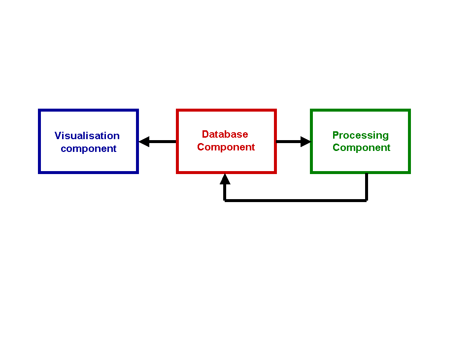
The DSS has three major components that need to be implemented in the design and are shown in Figure 7.
Each phase of the design will be discussed individually and the processing needs and requirements will be outlined. The actual design and implementation will need more thought than is shown in this document as a more accurate idea of the exact specifications should be known. This section, however, will give a breakdown of the processing requirements and the tools best suited to fulfil the purpose.
Figure 7 Major components of the DSS design
11.1 Database Structure
In this document the database used will be referred to as a generic structured database. It will perform two main functions, which are
The most important attribute of the database is that it needs to be able to store:
To achieve these goals it is necessary to look at the latest available technology that allows for flexibility in the data storage. Unfortunately, at present, there is no system that is able to link spatial data with time series data and a viewing platform in GIS. The database used by the ArcView GIS is dBase file format.
This requires the data storage in a flat file format that can produce a large amount of redundancy, and is not easily queried. A relational database has the ability to reduce redundancy and allow for easier query options to be developed. The ARC/INFO and ArcView systems are being developed to incorporate relational database facilities, these are however not available at present.In order to achieve this requirement of linking spatial, time series and attribute data together, it is necessary to link a GIS with a relational database. This methodology will allow the user to store attribute, time series (simulated and observed), and spatial data together in an accessible and functional format.
The BASINS system used in the USA has been designed to perform a similar operation to that described above, linking time series data with the ArcView GIS, using the WDM database. While it may appear the using an existing system such as the BASINS system which has been developed in the USA to perform the database functions is ideal there are several problems with using such as system which have been outlined in Section 10.1. When having a look at the option of using an existing system it is necessary to weigh up
In the time frame of this project using a system such as BASINS will require an enormous amount of time to translate South African variables into those that are compatible with those used in the USA. It also brings with it all the concerns raised in Section 10.1 and ties the modeller down to one specific model. It was believed that for the purpose of this project it would be better to look at local efforts in terms of database development and use already constructed systems which can be conformed to and enhanced. This allows for less requirements in terms of translating the different variables into usable quantities and also allows more flexibility in post development support and modification as there is no dependence on development skills in other countries who’s system you are tied in with.
The database design will therefore take on the form of a coupled system, which will link a relational database to the ArcView GIS. The databases that have been proposed for use consist of various relational databases include
The design of the database system is aimed at a PC platform. It appears the Oracle ArcView coupling looks like the most promising option in producing a spatial relational database link. The DWAF Geohydrology department is using the Regis, data storage system which already employs the ArcView Oracle link. There are some limitations especially in terms of the number of simultaneous access points that can be used by the access system and its inability to handle extremely large datasets. It is therefore clear that the other options such as SQL, Oracle and Informix offer the best opportunities in terms of database development.
The database design will follow the standards produced by the integrator, making sure that the database structure and architecture conform with the DWAF standards regardless of the database chosen to store the data. In such a case the system can be relatively easily translated if the data needs to be stored in another database at a later stage.
The database will house the data through a linked table format that associates a set of attribute or time series data to a spatial attribute code. The spatial attribute code, will then link to the GIS through a linked table which contains the spatial attribute code and the GIS attribute code which is associated to the data stored in the GIS. This format allows a "many to many relationship" to be used in the database and link the attribute and time series data to the GIS data. This feature should also allow the manipulation of spatial data and its associated attributes.
The construction of a spatial database that links GIS with a relational database is a time consuming process and needs much consideration on the specifics of how the data is going to be stored. This aspect is beyond the scope of this design as it requires more specific information. The database should conform with the standards proposed by DWAF as far as possible and should use the full range of capabilities afforded by linking a GIS to a relational database. The most likely storage facility to use would be the Arcview GIS linked with an Oracle database and most of the programming will probably done using Visual Basic coding as this is the new base language for ArcView 8. Regis and other systems presently used in DWAF will need further examination to prevent the duplication of effort.
The data stored in the database can further be classified into invariant and variant data (Figure 8). Invariant data is data, which comprises of mainly attribute data that will remain constant throughout a particular simulation or set of simulations such as soils and topographical data. Invariant data can include other data that can change over time, such as rainfall and temperature data, but remain constant for the simulation scenarios being tested.
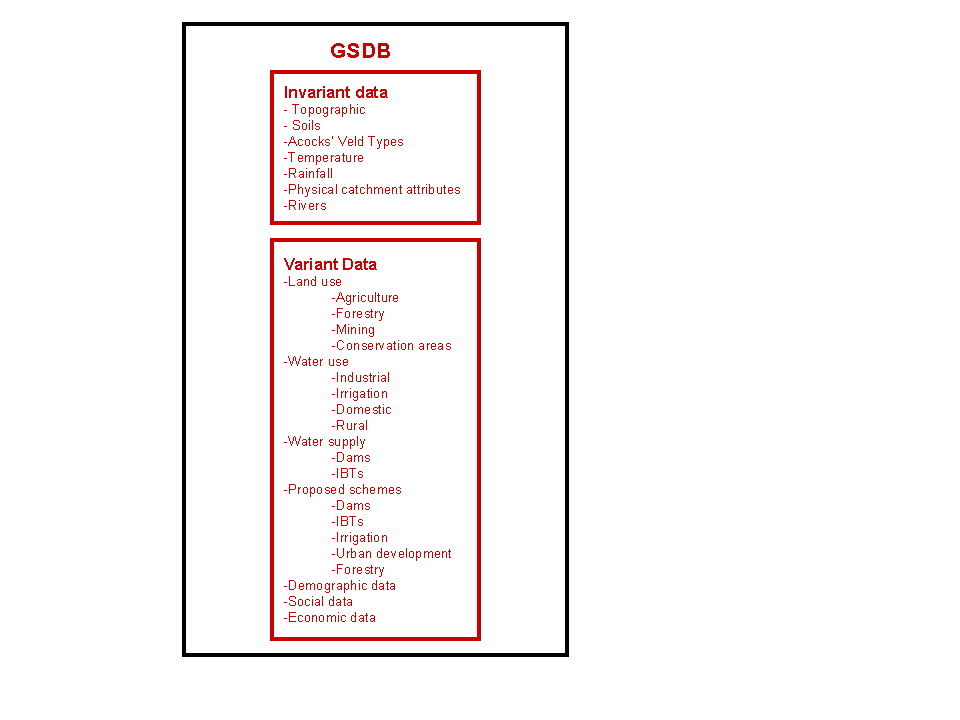
Figure 8 Some of the invariant and variant data requirements for the DSS
Variant data (cf. Figure 8) could be defined as data that can change dynamically over time or from scenario to scenario and is essentially land and water use data. Variant data also includes planning data such as the proposed constructions of new schemes. Simulated data is essentially variant data that also needs to be housed in the database. All the data should have a spatial component attached and be linked with the GIS.
Invariant data can be parameterised and placed into a model directly through the use of an attribute builder, which converts data from the database into parameters that can run the model. The variant data however might need to be manipulated and go through a transformation process before it is incorporated into the model. This could be done through the use of a Scenario Generator, which could be used to manipulate and change the initial primary data. An attribute builder could then be used to transform the data into parameters used by the model. The models once run also produce variant data, which will need to be stored in the database for query in the visualisation process. The processing required to perform these functions will be discussed in the next section.
There are several different processing requirements needed in the DSS. Initially there is the need to convert data from the database to the required format of different modelling tools being used in the DSS. This initial phase includes the attribute builder and Scenario Generator (SG).
The second level of processing occurs in the models themselves and manipulates the various inputs into the outputs required from the models. The third stage of processing is the transformation of model outputs back into a format suitable for the data storage.
The final level of processing required is the visualisation component and is the interpretation of both stored base data and stored generated (simulated) data into indicators that the decision maker can use. The first three phases will be addressed in this section and essentially deal with the primary processing components and not the visualisation.
Figure 9 is a systematic diagram showing the processing component and how it is linked to the database component of the design. The SG and attribute builder combine to manipulate the data into a format that is suitable for use in the different models. From the figure it can be seen that the invariant data feeds straight into the attribute builder, which feeds into the different models and tools. The variant data is transformed through a SG and is then fed into the attribute builder to be processed in the different models. The SG therefore allows the user to manipulate the invariant data changing it to suit the scenarios that need to be tested. The SG and the attribute builder are inextricably linked and are the basis of the processing component as they provide the input data for the different modelling tools.
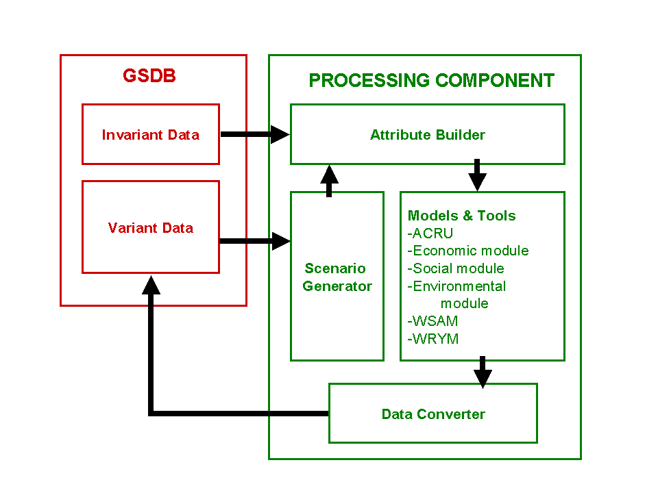
Figure 9 The processing component of the DSS
11.2.1 Scenario Generator and attribute builder implementation plan
The development of the SG will require the seamless integration of ArcView (or a similar suitable GIS package), the new ACRU model and other modelling tools being used in the DSS, and a relational database.
There are several large challenges that need to be addressed in the system integration:
The SG could be used for the testing of individual licenses where it is already known what type of development is being instituted or addressed and also used to incorporate planning scenarios where the information may need to be processed before the chosen scenarios can be run. For example population projections may need to be modelled to determine future water use in some areas.
In this phase the DSS will be compiled in such a way that different scenarios can be quickly and effectively generated using Graphical User Interfaces (GUIs). This section requires the seamless integration of several models including the economic and hydrological systems, which, once the user has defined the inputs, will run in the background to produce the results. The outputs will then be generated using GUIs with different indicators showing the results of the scenarios. This is, however, addressed in the visualisation phase. Both the inputs and outputs could be spatially referenced with outputs given in GIS format. The seamless integration is a time consuming process and would need to be programmed using an object orientated programming language. This way future changes or additions could be made relatively easily. It has been suggested that Visual Basic be used as the programming language as it interfaces with most Microsoft office applications.
The attribute builder takes the output from the both the SG and the database directly in the case of invariant data as shown in Figure 9. The attribute builder allows for the quick setup of certain parameters that need to go into the model directly. These parameters can be obtained from the database in terms of invariant data but may need manipulation using a GIS before they can be placed in the model. The processing and manipulation of this data may be time consuming, it is therefore recommended that in the case of the invariant data that these manipulations could be reduced if the actual parameter data is stored in the database directly after manipulation and is only changed using the attribute builder if the data is updated or a change in the model configuration is needed.
The SG information will however still require the full manipulation. The attribute builder needs to perform both GIS manipulations as well as plain programming processing. It has been recommended that the new ArcView 8 system be used to perform the GIS manipulations and that the Visual Basic programming language could be used as the base programming language to process the data and develop the GUIs needed in both the inputs required for the SG and the attribute builder. It is recommended that the outputs from the attribute builder should be produced in XML format, which is highly versatile and is easily transformable into other types of data formats needed to feed the model as well as giving the option of automated error checking. It has also been suggested that the menu format that will be used for the new ACRU is the XML. There are however several different types of modelling required in the processing phase of the DSS, which will be discussed in the section to follow.
11.2.2 Modelling tools required in the processing phase of the implementation plan
Hydrological, economic, social and ecological modelling will be required to be performed using the DSS in the processing phase as detailed in the following sections.
The hydrological modelling component will be performed mainly with the use of the new ACRU modelling system. This system is currently under development and at a later stage will be able to perform process based hydrological modelling that is able to address the operational hydrology in a system and water quality concerns.
The DSS, however, is not tied to one modelling system and more hydrological models could be used if necessary. It will, however, be necessary to write a transformation routine (attribute builder) for any new models that would be added on. The DSS structure, which is shown in Figure 9, is not model dependent. New models can be added to the system when and where appropriate. The database therefore could be used to provide data and house simulation results from a number of different models such as WRYM and WSAM.
Developing an economic modelling component that combines feasibility criteria, yield potential and economic viability in a spatial framework is required. This will allow a decision maker to better understand the economic implications of particular land use management practice scenarios.
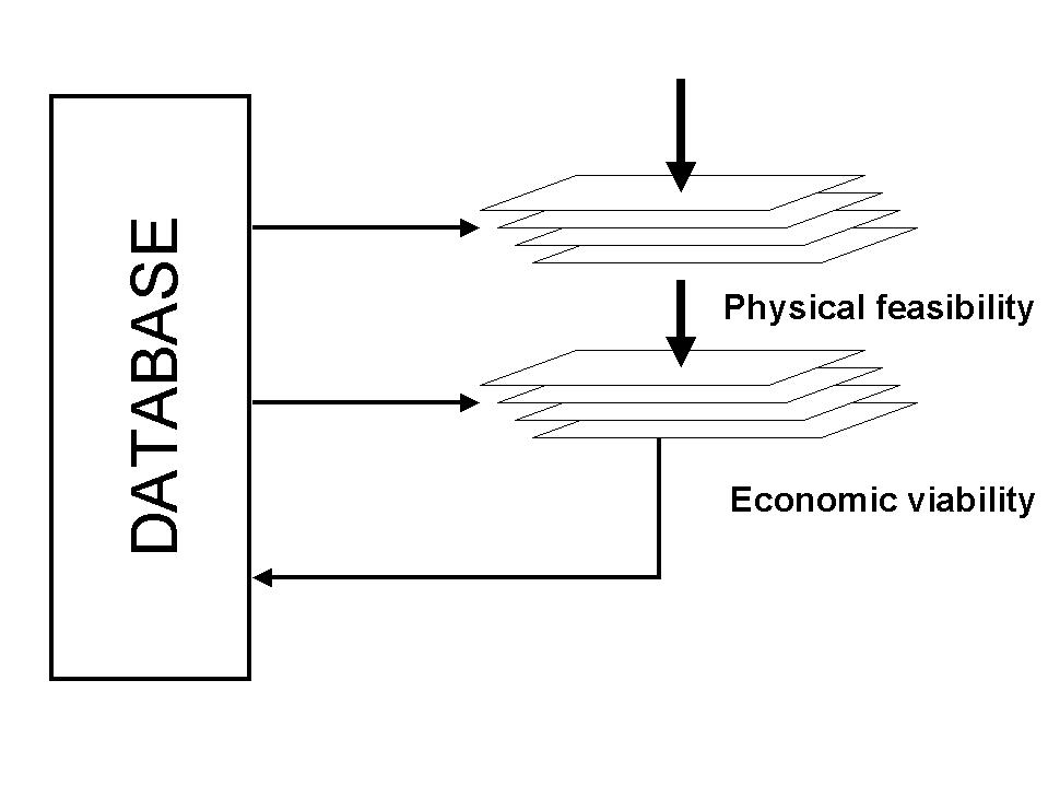
Figure 10 Economic modelling component of the DSS
The feasibility of growing a specific crop in a specific place is a combination of a number interacting climatic and geophysical factors. In order to determine the feasibility of growing crops in certain locations requires both climatic and topographic data along with the crops biophysical requirements.
A spatial representation of the yield potential could then be obtained by extracting both topographical and climatic data from the database in a GIS format. The different biophysical factors such as temperature, rainfall, soil depth and aspect, can then be weighted in a linear algorithm, which could then be used to determine the physical feasibility of growing a crop in a particular place. This is effectively equivalent to placing a number of different layers of spatially referenced information over one another manipulating each layer according to certain criteria to determining the potential crop yields in these areas (Figure 10).
In the initial feasibility study crop potential could be determined using the growing degree day concept, where yield potentials will be determined by the average temperature and rainfall conditions. They could be determined by the use of a crop growth model. The ACRU model is able to produce some estimates of crop yields but not the full range that may need to be looked at. It may be necessary to use a model that has been specifically designed to do crop modelling in this component of the study. Areas where crop growth is extremely unlikely will be excluded from the potential crop growth areas using a filtering process. While an area may potentially support a wide variety of crops other factors such as distance from markets and transport routes may restrict a specific crop’s economic viability. Even if a crop can grow in a specific area it does not mean that it is economically sound to do so.
Once the physical feasibility of growing specific crops in certain areas has been determined, the economic viability of doing so must be investigated. Economic information thus also needs to be combined with the crop yield potential to determine the economic viability of growing a selected crop in the area. The database will hence also need to contain continuously updated data on crop sales prices both nationally and internationally, as well as value added information such as processed product costs, transport costs and number of people employed. This aspect of the economic component of the DSS will require both the manipulation of spatial referenced data and pure data. Spatial information will comprise of different aspects such as access to markets due to distance from transport routes, distance from the river in terms of irrigated agriculture amongst other spatial data. This section will take on a similar form to the physical viability as different layers of information will be given weightings that will help to determine the economic viability (Figure 10). Initially a filtering process will be used to eliminate areas that are totally unviable.
This will require a multidisciplinary team, including GIS, economic, hydrological and agronomic expertise. The initial system will be set up to account for a broad range of crops with only a few different genus included for the larger species. The database can be modified when more information is required.
This component will again consist of the use of both GIS technology and regression modelling. It will allow for a similar structure of that in the economic modelling component which has several different layers of information that are draped over each other with certain specific weights to produce social information that could be used to generate indicators that could aid the decision maker.
In this design the main concentration has been on the hydrological and economic modelling. Further studies are on the way to collect and determine specific social values that could be used to aid water managers and decision makers in assessing different water uses in terms of the equity, efficiency and sustainability criteria outlined in the NWA (1998). These could then be used in the SG to aid the development of different scenarios, which can be easily tested.
Ecological variables could be determined in much the same way as those in the economic and social modelling components. This component will require extensive GIS modelling where layers of information, such as biodiversity and conservation areas, could be draped together with different weights to determine certain ecological indices.
These indices could then be used to limit certain scenarios in the SG. Some ecological data will be generated in the hydrological modelling where impacts on the ecological reserve could be estimated. The ecological modelling is a subset that needs to be considered in the main structure of the DSS but is not the focus of the initial development, which is concentrating on economic and hydrological modelling.
The visualisation component consists of two main aspects (Figure 11). The initial part is the translation of variables produced by simulation scenarios and base data into indicators that could be used by the decision maker and the second aspect is the display system used to display the different indicators in a suitable format that can be used by the decision maker.
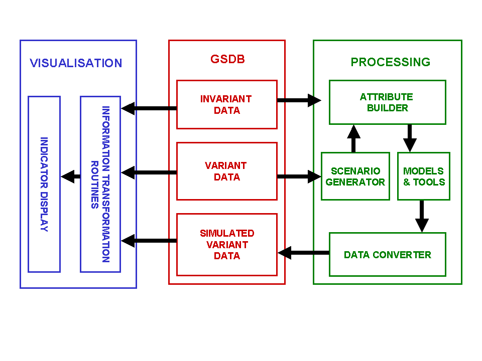
Figure 11 The visualisation component of the DSS and the linkages to the database and processing components
Before either of these phases can be embarked upon it is necessary to determine the types of indicators needed by the decision makers and stakeholders. This process will require a lot of consultation between the various parties involved in CMAs. Once a generic set of indicators has been defined the system could be put into place to generate the indicators from the database and visually display them.
The display format would need to combine GIS with other systems and be able to display results at certain points in the catchment of interest. It is recommended that the ArcView 8 system be used for display purposes. This could tie the use of the DSS to the ArcView format.
It was suggested that other display options such as Map Objects be considered for display purposes, however, the manipulation functions available in Map Objects are limited. The data manipulation needs to process both vector and rasta data this is not available in the Map Objects system.
The most likely programming language to be used for the visual display option is Visual Basic as it is designed specifically for display purposes and it is able to communicate via Visual Basic application programming to the ArcView 8 system as well as most Microsoft applications. The summarisation and translation of variables into indicators could be performed with any programming language, however, in the interests of consistency Visual Basic should perhaps again be used.
The visualisation component is exceptionally important (as it is the information provided by this component that the user will base a decision) in the system design and will need to be comprehensively thought through before embarking on any coding begins.