The entire basis for Predictor Corrector methods rests on Taylor's theorem, so for convenience let us restate it here...
Taylor's theorem states that for any mathematically "nice-and-smooth"
function Y(t), (where "nice-and-smooth" can be given a highly technical and
precise meaning), the following is true.

Where ![]() is an unknown value anywhere from t to
is an unknown value anywhere from t to ![]() .
.
Now by experimentation I found that a second order PECE method worked best for this particular problem, so I will only show the derivation of a second order method.
Firstly a few concepts and a bit of notation.
A differential equation solver estimates the solution to the equation at certain times.
Traditionally this was done on the basis of a fix time step. In times when little is
happening, one can take large time steps, and in times of flood, one must take small time
steps. Thus with fix time step methods one must fix the time step small enough to cope
with the worst conditions. This resulted, for this model, in unacceptably long run times.
Denote the time at which the i'th value is calculated by ![]() . Denote the i'th
time step
. Denote the i'th
time step ![]() by
by ![]() .
.
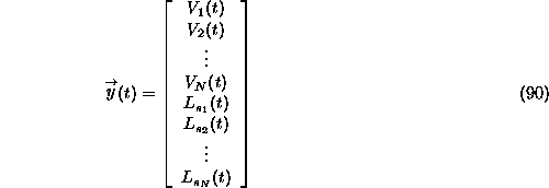
The state of the lake is determined by the ``state'' variables. ie Salt load in each
cell and water volume in each cell. For the purpose of solving the differential equations
we have no need to know what the state variables are. Thus if we have an N cell lake model
we would define the state vector to be a 2N dimensional vector ![]() :-
:-

Then the differential equations can be written in the form :-
![]()
Denote the value the state vector at time i by ![]() . Note that this isn't
the i'th component of the state vector, but the state vector at time i. Denote the n'th
derivative by
. Note that this isn't
the i'th component of the state vector, but the state vector at time i. Denote the n'th
derivative by ![]() .
.