Very simplified version for analytic solution.

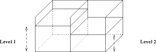
Referring to equation 1, and figure 10, assume two equal sized square sided cells. Thus the areas and the levels , where is the volume of the i'th cell.

  
Figure 10: Two square sided cells of equal area.

So the flow from cell 1 to cell 2 is ...

Assuming no in or out flows, only the inter-cell gravity link...

Placing this in matrix form...

Where

Now find the eigenvectors and eigenvalues of the matrix so that one can diagonalize the matrix. An eigenvalue of a matrix B and its corresponding eigenvector is defined to be such .

Thus the determinant of must be zero, this gives you the characteristic polynomial

Solving the characteristic polynomial, we get the eigenvalues and . Using these to find the corresponding eigenvectors we get and thus we can diagonalize the matrix.

Perform a change of variable to variables that are basically the eigenvectors of the problem. ie let and .

Then...

Thus is a constant of the system. (No surprise, this is just saying that , the total volume of water in the system is conserved.)

And ...

Which is now an equation which we can solve...

Integrating both sides gives us...

Where K is an arbitrary constant of integration.

Taking the exponential of both sides and letting gives us...

Where is an arbitrary constant of integration to be determined by boundary conditions.

Now reversing the substitution of variables we have...

Now at time t=0 we have...

Solving for the constants and we get...

  
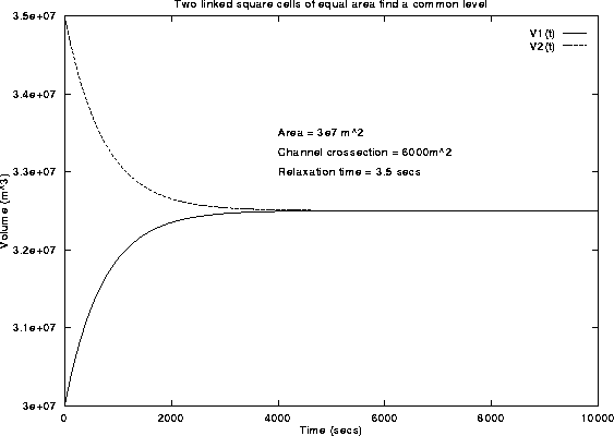
Figure 11: The volumes in two linked cells reach common level. The parameters are chosen to be similar to the North Lake cell.

Which finally gives us the exact analytic solution for this trivialised problem. See figure 11 for a graphical representation.

Volume of two linked square sided cells of equal area.

 

So what can we learn from the solution?

• The solution consists of the sum of two solutions.
• One of which corresponds to eigenvalue 0. This corresponds to the conservation of total volume.
• The other is an exponential decay term.
• The volumes tend to the average value as t tends to infinity.
• The level difference is never wiped out. 
• I took the matrix approach because it can easily be generalized to n cells of different size. If you do this the above points generalize to :-
  • The solution consists of a sum of N solutions.
  • At least one of which is a constant. (Again the conservation of total volume.)
  • The rest are exponential decay terms of various rates.
  • The decay rates are the eigenvalues of the matrix.
  • The levels tend to a weighted average value as t tends to infinity.
  • The level differences are never wiped out.

• The Relaxation time and the half-life.